install.packages("galah")
library(galah)
galah_config(email = "your@email.com")Where the turtles roam? Sea turtle sighting patterns around Australian coastlines
R
Marine biology
Data visualisation
Open data

Why turtles 🐢
I grew up facinated by ocean animals and Australia’s marine biodiversity has always felt like something worth paying attention to.
While Australia is the home to six of the world’s seven sea turtle species, making it a global hotspot for these fascinating marine reptiles. The green turtle, loggerhead, hawksbill, olive ridley, flatback, and leatherback all swim through Australian waters at some point in their lives. One of them, the flatback nests exclusively on Australian beaches and nowhere else in the world.
The project started from a simple question: Where do turtles actually go, and when?
The data
The data for this project comes from the Atlas of Living Australia (ALA), Australia’s national biodiversity database. First introduced to me during the Wild-Caught Data unit at Monash University, the ALA aggregates species occurrence records from researchers, scientists, museums, and agencies making it one of the richest open biodiversity datasets available for Australian species.
To access the data in R, I used the galah package (the official R package for the ALA). It allows direct querying of the ALA database without manual downloads, making the analysis fully reproducible.
Rather than pulling one species at a time, I queried at the family level using Cheloniidae which is the scientific family that covers all hard-shelled sea turtles. This captured all five species of interest (green turtle, loggerhead, hawksbill, olive ridley and flatback) in one single query. Then, the query is filtered from the year 2000 onwards to focus on the modern monitoring period, where data quality and coverage is more consistent. Earlier records exist but are sparse and less reliable for spatial analysis.
The fields selected cover the essentials for this analysis: - scientificName to identify the species - decimalLatitude and decimalLongitude for mapping - eventDate, year, and month for temporal analysis
all_turtles <- atlas_occurrences(
  identify = galah_identify("Cheloniidae"),
  filter = galah_filter(
    year >= 2000
  ),
  select = galah_select(
    scientificName,
    decimalLatitude,
    decimalLongitude,
    eventDate,
    stateProvince,
    year,
    month
  )
)
The raw dataset returned a mix of family-level records, subspecies entries, and genus-only records alongside the five main species. I retained only records identified to species level:
library(dplyr)

clean_turtles <- all_turtles %>%
  filter(scientificName %in% c(
    "Caretta caretta",
    "Chelonia mydas",
    "Eretmochelys imbricata",
    "Lepidochelys olivacea",
    "Natator depressus"
  )) %>%
  filter(!is.na(decimalLatitude),
         !is.na(decimalLongitude),
         !is.na(year)) %>%
  mutate(species_common = case_when(
    scientificName == "Caretta caretta" ~ "Loggerhead",
    scientificName == "Chelonia mydas" ~ "Green turtle",
    scientificName == "Eretmochelys imbricata" ~ "Hawksbill",
    scientificName == "Lepidochelys olivacea" ~ "Olive ridley",
    scientificName == "Natator depressus" ~ "Flatback"
  ))
I also filtered the coordinates to valid Australian bounds, removing a small number of clearly erroneous entries including points plotted outside Australian waters, and restricted the year range to 2005 to 2024.
clean_turtles <- clean_turtles %>%
  filter(
    decimalLatitude >= -45,
    decimalLatitude <= -10,
    decimalLongitude >= 110,
    decimalLongitude <= 155,
    year >= 2005,
    year <= 2024
  )
2013 shows an unusually high spike of around 40,000 records, likely a bulk historical upload to the ALA rather than a genuine surge in sightings. It is retained but worth keeping in mind when interpreting trends over time.
The final dataset contained 147,811 records across five species, covering Australian coastlines from 2005 to 2024.
------The analysis
Where do they appear?
The map below plots all sightings coloured by species, revealing immediately that turtle distribution is anything but uniform.
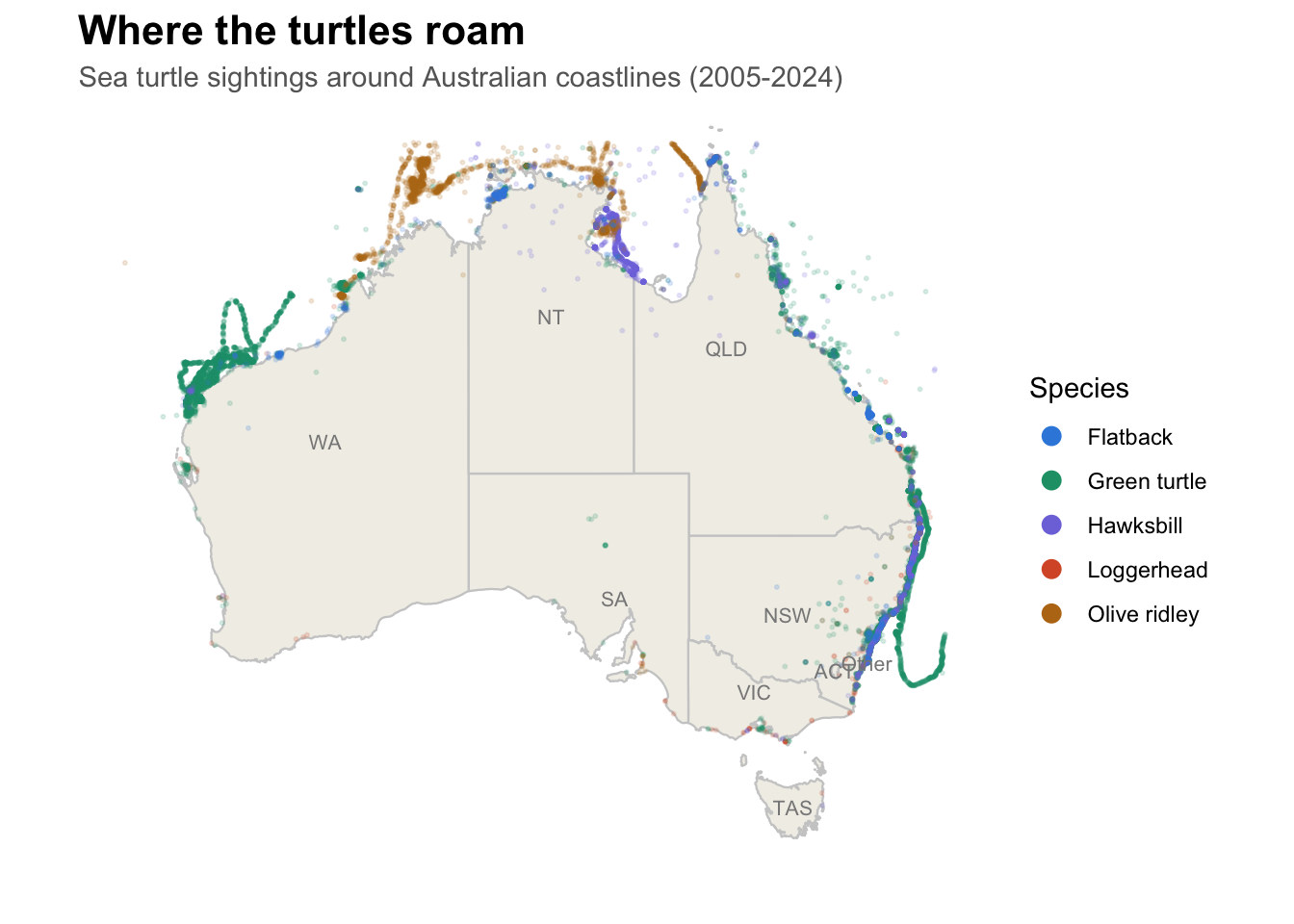
Western Australia dominates the sighting count with over 90,000 records. The long curving lines of green turtle tracks tracing migration paths along the coast are a striking feature of the map.
Queensland’s Great Barrier Reef is a hotspot for multiple species clustering along the eastern coastline. The tropical north is where the rarest species concentrate, while the south is almost entirely empty. Turtles are fundamentally tropical animals and their distribution reflects this clearly.
Some of the long curving lines visible along the WA coast are not separate sightings. They are the tracked movements of individual turtles wearing satellite tags. A single tagged turtle swimming up the coast generates dozens of location points, which plot out as a trail on the map. This is a good reminder that the data comes from many different sources. Some records are one-off sightings reported by members of the public, while others are continuous tracking data from research programs following specific animals over time.
When do they appear?
The second question was temporal: does each species follow a different seasonal pattern? The short answer is yes and dramatically so.
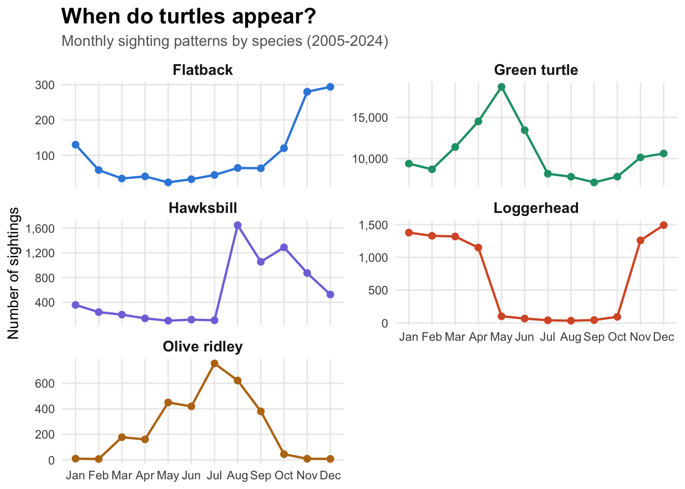
The faceted chart reveals five distinct seasonal signatures.
The flatback and loggerhead both peak sharply during the nesting season window of November to January. These species come ashore to breed during the Australian summer.
The green turtle peaks in May, well after nesting season, suggesting these sightings reflect feeding migrations rather than breeding activity.
The hawksbill and olive ridley both peak in the Australian winter (from July to September) a pattern that sits entirely outside the nesting window and likely reflects seasonal feeding movements into warmer northern waters.
To make these differences even clearer, the heatmap below scales each species independently, showing relative activity rather than raw counts.
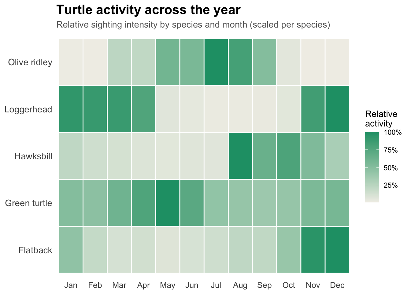
The loggerhead’s near-complete disappearance from May to October stands out starkly against the green turtle’s year-round presence. The olive ridley’s winter peak is the most visually distinct pattern of all.
Do they keep its own calendar?
The amber bands mark the nesting season (November to January) when female turtles come ashore to lay eggs on Australian beaches. But not very species follows that rhythm.
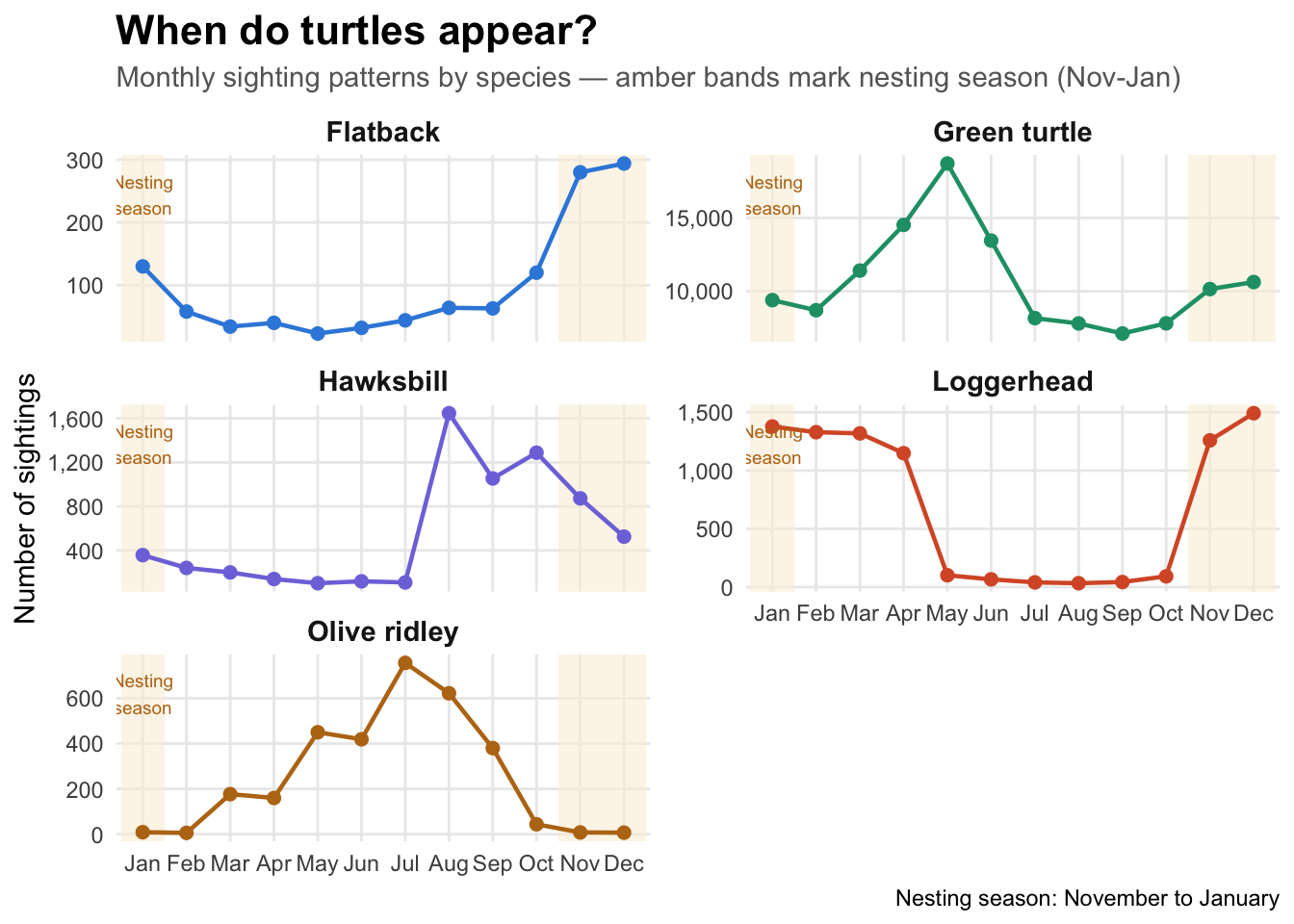
The loggerhead shows the clearest nesting signal. Sightings are high from January through April, drop almost to zero through the middle of the year, then surge again in November and December. The pattern is almost symmetrical around the nesting season window. These turtles appear when it is time to breed and largely disappear in between.
The flatback tells a similar story. Quiet for most of the year, it builds steadily from October and peaks sharply in November and December, right inside the nesting window. For Australia’s only endemic turtle, the data confirms what biology predicts.
The green turtle is different. Its peak falls in May, well after nesting season has ended. The elevated counts across most of the year suggest these sightings reflect feeding migrations rather than breeding activity, with green turtles travelling along the coastline in search of seagrass beds.
The hawksbill peaks in May and again in August to September, outside the nesting window entirely. This mid-year pattern is the least intuitive of the five and likely reflects seasonal feeding movements into warmer northern waters.
The olive ridley is the most striking outlier. Its peak sits firmly in July and August, in the middle of the Australian winter, and it almost vanishes during the nesting season. Of all five species, the olive ridley appears to operate on a completely different seasonal calendar from its relatives.
Together these five patterns tell a story that raw numbers alone cannot: same ocean, same coastline, five completely different relationships with the calendar.
What the data is really telling us
The 147,811 sightings in this dataset did not appear automatically. They were logged by researchers attaching satellite tags to nesting females, by citizen scientists submitting observations through wildlife apps, by park rangers conducting systematic beach surveys, and by volunteers counting turtle tracks at dawn.
The patterns visible in the data, the seasonal rhythms, the geographic hotspots, the differences between species, are ultimately a product of where humans chose to look and how consistently they looked. Western Australia’s dominance in the sighting count reflects both the length of its coastline and the presence of active long-term monitoring programs like those at Ningaloo Reef.
This does not make the analysis less valid. It is simply a reminder that open biodiversity data is shaped by human observation effort as much as by the animals themselves. The map shows where turtles were seen. It also quietly shows where people were looking.